Using Autofilters in Microsoft Excel
Following a hefty chunk of data analysis the last few days, CTRL + SHIFT + L has probably been my most used shortcut this week. This activates data filters on your Excel spreadsheet – alternatively you can switch them on and off by going to Data then Filter on the ribbon (or toolbar pre Microsoft Office 2007). THe shortcut however really comes into its own on toggling the filters on and off, saving time clearing them each time.
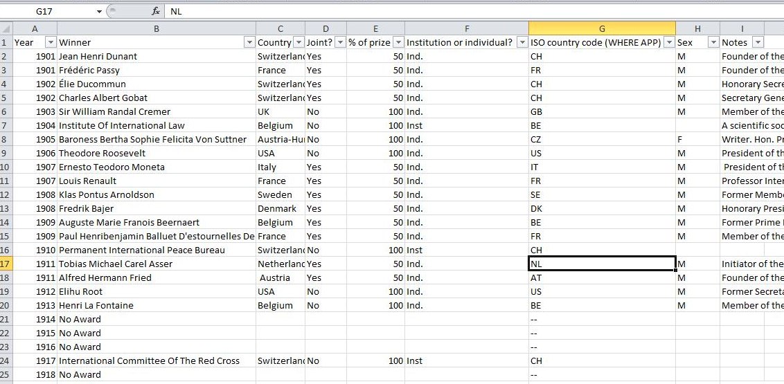
If you’re not already familiar with filters then I thoroughly recommend you check them out, data filters (or autofilters) are a simple way of helping drill down through your data. Take for example the following spreadsheet which is based on the Nobel Peace Prize winners (taken from the Guardian’s DataBlog)
Let’s assume that to start with we wanted to just drill down to find out who were the UK winners. Activate the filters by either using the shortcut or by going to Data on the ribbon and choosing the filter option on versions 2007 and 2010.
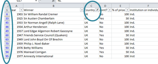
By using the data filter we can click on the little arrow on the country column and select just the UK. Suddenly all other data becomes hidden and only those winners from the UK are shown.
You can see that the filter has been activated because there is a small filter symbol rather than an arrow (to indicate which column has been filtered). In addition the row numbers are also highlighted in blue (see the pic above). If you want to you can also drill down further by using other filters, for example to see which UK institutions have got the award just use the filter on column F, “institution or individual”.
Sometimes though you can get carried away with layering multiple filters on different columns and as I said above, this is where the shortcut really comes into its own. Rather than having to go through all the filters to uncheck them if you wish to go back to display all data in the original list just use CTRL+SHIFT+L to toggle the filters on and off.
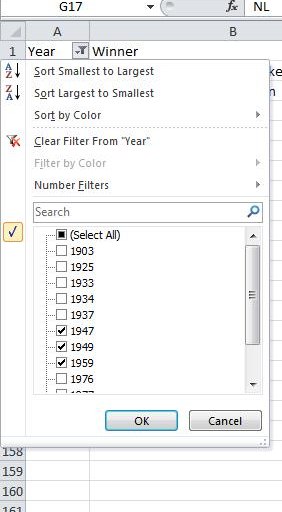
Don’t forget to have a play with some of the other options on the filters – in Excel 2007 and later versions you can use multiple options to drill down, selecting for example particular years by checking and unchecking boxes:
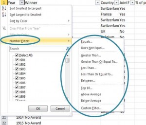
You can also use the autofilters to pull out data such as the top 10 largest values, or values between certain criteria – choose the Number filters option and then select which options you’re after.
 Just a few suggestions here but using the data filters are a brilliant way to help you pull out particular strands of data or groups on your spreadsheet, do give it a try: CTRL + SHIFT +L
| Print article | This entry was posted by Jennifer Deacon on December 2, 2011 at 3:25 pm, and is filed under Excel Hints, Keyboard Shortcuts. Follow any responses to this post through RSS 2.0. Both comments and pings are currently closed. |
Comments are closed.


