Posts tagged excel

Using Autofilters in Microsoft Excel
Dec 2nd
Following a hefty chunk of data analysis the last few days, CTRL + SHIFT + L has probably been my most used shortcut this week. This activates data filters on your Excel spreadsheet – alternatively you can switch them on and off by going to Data then Filter on the ribbon (or toolbar pre Microsoft Office 2007). THe shortcut however really comes into its own on toggling the filters on and off, saving time clearing them each time.
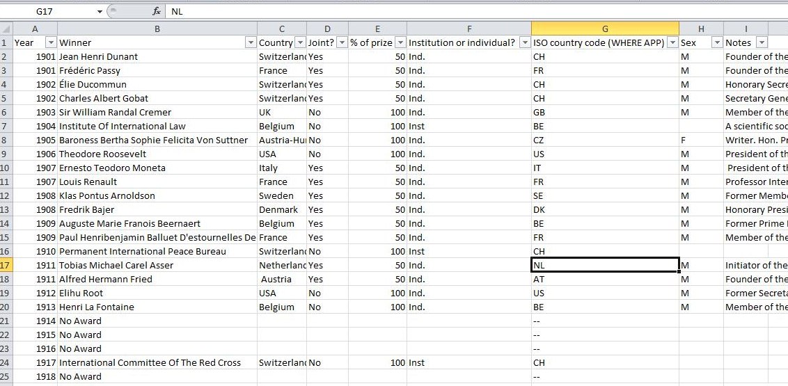
If you’re not already familiar with filters then I thoroughly recommend you check them out, data filters (or autofilters) are a simple way of helping drill down through your data. Take for example the following spreadsheet which is based on the Nobel Peace Prize winners (taken from the Guardian’s DataBlog)
Let’s assume that to start with we wanted to just drill down to find out who were the UK winners. Activate the filters by either using the shortcut or by going to Data on the ribbon and choosing the filter option on versions 2007 and 2010.
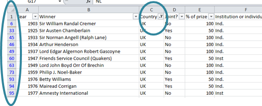
By using the data filter we can click on the little arrow on the country column and select just the UK. Suddenly all other data becomes hidden and only those winners from the UK are shown.
You can see that the filter has been activated because there is a small filter symbol rather than an arrow (to indicate which column has been filtered). In addition the row numbers are also highlighted in blue (see the pic above). If you want to you can also drill down further by using other filters, for example to see which UK institutions have got the award just use the filter on column F, “institution or individual”.
Sometimes though you can get carried away with layering multiple filters on different columns and as I said above, this is where the shortcut really comes into its own. Rather than having to go through all the filters to uncheck them if you wish to go back to display all data in the original list just use CTRL+SHIFT+L to toggle the filters on and off.
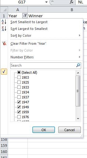
Don’t forget to have a play with some of the other options on the filters – in Excel 2007 and later versions you can use multiple options to drill down, selecting for example particular years by checking and unchecking boxes:
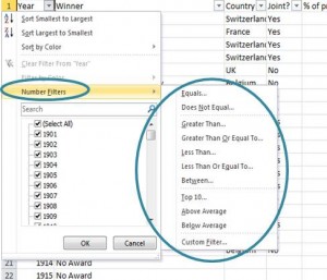
You can also use the autofilters to pull out data such as the top 10 largest values, or values between certain criteria – choose the Number filters option and then select which options you’re after.
 Just a few suggestions here but using the data filters are a brilliant way to help you pull out particular strands of data or groups on your spreadsheet, do give it a try: CTRL + SHIFT +L

Removing line breaks within a cell
Nov 18th
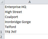
Did you know that you can put line breaks inside excel cells? It’s quite straight forward, within the cell just click ALT + Enter to make the line break. An example is if an address is entered in a single cell:
Personally it’s not something that I would use often as it makes the data harder to extract and analyse, but what happens if you have a spreadsheet has these incell line breaks, and need to break them out into columns? In the example here you may want to do an analysis on the geograhic spread or want to do a mail merge so want a list with columns for towns, counties etc.
If the lines were in separate cells you could use the paste special > transpose option to convert vertically listed data items into horizontal and vice versa however in this instance it won’t work as all the data is in a single cell. Instead what we need to do is remove the line breaks.
Using ALT + ENTER means that Excel inserts a line feed character, or ASCII CHAR(10) which shows as a new line. We need to remove these instances of CHAR(10) which appear invisible on screen and replace them with something else to act as a delimiter which we can then use to break the data into columns.
- To start with add a new helper column on your spreadsheet, in this instance it would be column B and type the formula =SUBSTITUTE(A1,CHAR(10),”£”)
- Fill this formula down against the rows that you have. This formula searches the cell indicated (eg cell A1) for all instances of CHAR(10) and substitutes them with £
- You can then use the Text to Columns function to break the data into columns using £ as the delimiter. You can of course use any character you like rather than the £ however make sure that it’s something you know doesn’t already appear in your data as otherwise the columns may break in the wrong places. And watch out for using the wildcard characters too (see my previous post on searching for wildcard characters)
The other alternative is to use find and replace to identify the line feed breaks which may be more appropriate if you have a large dataset with line breaks within the cells that need removing in a number of different columns. across the spreadsheet. However if you open the find and replace dialog box (CTRL + H) and type ALT + ENTER in the find box what happens? Erm, yes nothing – it just moves to the next box. Instead in the find box hold down ALT and type 010 then move the replace box and type in what you want the delimiter to be – eg £. Click Replace all and it should do the same as above but without the helper column.
Microsoft Excel Shortcut Tweet Roundup w/c 10th October
Oct 14th
In an almost unprecedented frenzy I blogged twice this week: once on wildcard searching in Excel, and also on finding out the day from a given date in a spreadsheet. As usual I tweeted a number of shortcuts which are as below, and was delighted to bump into someone this week who thanked me for tweeting the shortcuts, CTRL + K for hyperlink in particular. It’s good to know they’re being used! Here’s this week’s roundup:
_________________________________________________________________________________________
Toggle Office Ribbon CTRL + F1
Find CTRL + F
Replace CTRL + H
Open Text to Columns Dialog ALT + A then E
Select All CTRL + A
_______________________________________________________________________________________________
That’s it for me, I’m off to London to revisit some old haunts frequented before our move to Shropshire. Have a lovely weekend!

Finding the day of a week in Excel
Oct 13th
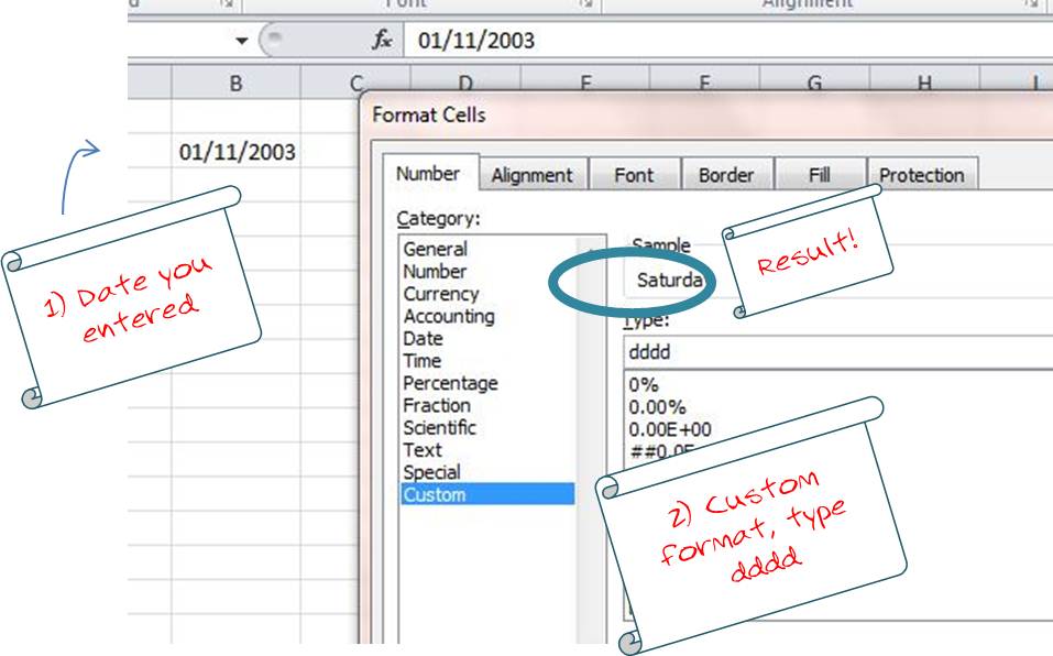
I read an article this morning on Lifehacker which outlined some ways to work out what day of the week a given date was. Clever as these methods are, if you’re by a computer you can do this through Excel as long as it’s for a date after 1st January 1900:
- Open a new spreadsheet or find a blank cell and enter the date eg: 1/11/2003.
- Making sure that the cell is selected open the format cells dialog (CTRL + 1)
- Select custom number format.
- Overwrite the entry in the type box with DDDD and you can see in the sample field that what the day of the week was.
Microsoft Excel Shortcut Tweet Roundup w/c 3rd October
Oct 7th
So this week’s Excel shortcut tweets turned out to be a celebration of F11:
______________________________________________________________________________________________
Insert a new worksheet SHIFT + F11
Delete the current sheet ALT + E then L
Activate Chart tool / wizard F11
Open VBA Editor ALT + F11
_______________________________________________________________________________________________
You may wonder what CTRL + F11 does. This inserts a new macro worksheet which is a relic back of the Excel4 days. Yes almost 20 years since Excel 4, when macros were written in a particular worksheet rather than the VBA editor, this shortcut still exists. As far as I know the new worksheets (titled Macro1 etc) don’t have any real use apart from for compatibility with the older version, unless you know to the contrary? Leave me a comment below as I’m intrigued if they’ve other uses.

