Posts tagged shortcut

Using Autofilters in Microsoft Excel
Dec 2nd
Following a hefty chunk of data analysis the last few days, CTRL + SHIFT + L has probably been my most used shortcut this week. This activates data filters on your Excel spreadsheet – alternatively you can switch them on and off by going to Data then Filter on the ribbon (or toolbar pre Microsoft Office 2007). THe shortcut however really comes into its own on toggling the filters on and off, saving time clearing them each time.
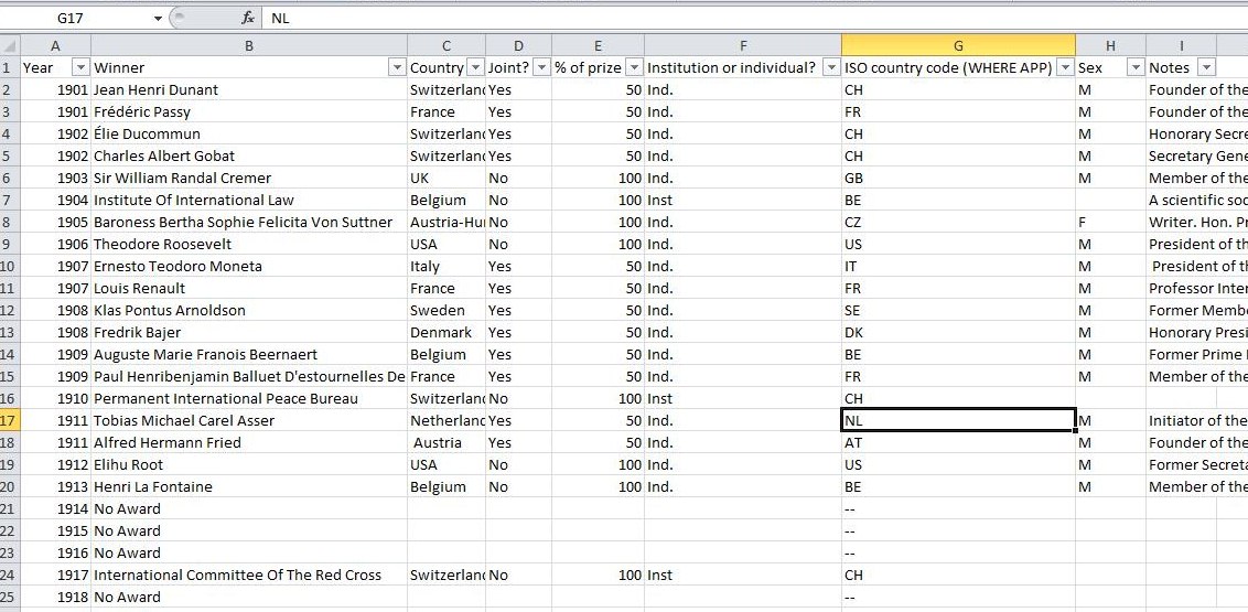
If you’re not already familiar with filters then I thoroughly recommend you check them out, data filters (or autofilters) are a simple way of helping drill down through your data. Take for example the following spreadsheet which is based on the Nobel Peace Prize winners (taken from the Guardian’s DataBlog)
Let’s assume that to start with we wanted to just drill down to find out who were the UK winners. Activate the filters by either using the shortcut or by going to Data on the ribbon and choosing the filter option on versions 2007 and 2010.
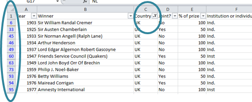
By using the data filter we can click on the little arrow on the country column and select just the UK. Suddenly all other data becomes hidden and only those winners from the UK are shown.
You can see that the filter has been activated because there is a small filter symbol rather than an arrow (to indicate which column has been filtered). In addition the row numbers are also highlighted in blue (see the pic above). If you want to you can also drill down further by using other filters, for example to see which UK institutions have got the award just use the filter on column F, “institution or individual”.
Sometimes though you can get carried away with layering multiple filters on different columns and as I said above, this is where the shortcut really comes into its own. Rather than having to go through all the filters to uncheck them if you wish to go back to display all data in the original list just use CTRL+SHIFT+L to toggle the filters on and off.
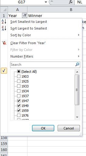
Don’t forget to have a play with some of the other options on the filters – in Excel 2007 and later versions you can use multiple options to drill down, selecting for example particular years by checking and unchecking boxes:
You can also use the autofilters to pull out data such as the top 10 largest values, or values between certain criteria – choose the Number filters option and then select which options you’re after.
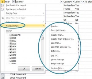 Just a few suggestions here but using the data filters are a brilliant way to help you pull out particular strands of data or groups on your spreadsheet, do give it a try: CTRL + SHIFT +L

Wildcard searching in Excel
Oct 12th
Reading a blog post solution prompted my two shortcut tweets today (I missed one yesterday, hence the extra!)
CTRL + F and CTRL + H open the Find and Replace tool respectively, both very handy shortcuts that I use frequently. You only need remember one as can then choose the tabs at the top of the dialog box to go to the one you need. Also handy that they are among those that don’t just work in Excel but across the Microsoft office suite in Word, PowerPoint and Access as well.
It’s a straightforward tool – there are a few options you can change when searching which I’ll save for a future blog post – but the post reminded me of my time in an office when we once needed to remove asterisks that had appeared in a set of data. My colleague’s first thought was to go straight to CTRL + H, activating the replace box and put * in the first box, leaving the second box blank, thus replacing it with nothing and in effect removing the pesky asterisks
But wait, what do you think happened? As * is used as a wildcard character to indicate any number of characters Excel assumed that they were looking for any characters and then removed them all, leaving a blank spreadsheet and a howling colleague. Quick use of CTRL + Z (undo) and the spreadsheet was returned to before.
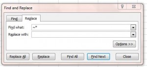
The solution: before the asterisk in the “find what” box use a tilde sign ~ before the asterisk: ~* This tells Excel that it’s an actual * that is being searched for and is not being used as a wildcard.
This should also be used if searching and / or replacing for a question mark ( ? is used as a wildcard indicating a single character) and if you’re actually looking for a tilde you’ll need to have ~~ in the find what box.
Hope that this is helpful, more information is in a microsoft knowledgebase here.

The power of Save As and your Excel spreadsheet
Sep 27th
I often tell people that F12 is one of the most useful keyboard shortcuts for any of the Microsoft products, including Excel, and certainly it is one of the ones that has been most useful to me. But why is Save As so important?
It’s simply a way of saving your spreadsheet or document in another way. This could either be with another name, or possibly into a different format (either a previous version of the software, or perhaps in an entirely different form such as pdf or .txt)
For me it’s using it to save a spreadsheet as another name which has been so useful, this gives the opportunity to have an “Original” version of a spreadsheet to return to whilst you try out some new functions and take your analysis in different ways with no fear of harming your source data. You can always return to the first version if needed.
Just a word of cation though, firstly make sure your new file names are meaningful and secondly that you don’t get click happy using F12 too often, ending up with multiple copies with helpful titles as “ORIGINAL Version 1 FINAL” or “Wednesday version 3 FINAL original use this one”.
Do you Save As and find it useful? What’s your favourite shortcut? Do leave me a comment below

