Excel Examples
Microsoft Excel Shortcut Tweet Roundup w/c 10th October
Oct 14th
In an almost unprecedented frenzy I blogged twice this week: once on wildcard searching in Excel, and also on finding out the day from a given date in a spreadsheet. As usual I tweeted a number of shortcuts which are as below, and was delighted to bump into someone this week who thanked me for tweeting the shortcuts, CTRL + K for hyperlink in particular. It’s good to know they’re being used! Here’s this week’s roundup:
_________________________________________________________________________________________
Toggle Office Ribbon CTRL + F1
Find CTRL + F
Replace CTRL + H
Open Text to Columns Dialog ALT + A then E
Select All CTRL + A
_______________________________________________________________________________________________
That’s it for me, I’m off to London to revisit some old haunts frequented before our move to Shropshire. Have a lovely weekend!

Wildcard searching in Excel
Oct 12th
Reading a blog post solution prompted my two shortcut tweets today (I missed one yesterday, hence the extra!)
CTRL + F and CTRL + H open the Find and Replace tool respectively, both very handy shortcuts that I use frequently. You only need remember one as can then choose the tabs at the top of the dialog box to go to the one you need. Also handy that they are among those that don’t just work in Excel but across the Microsoft office suite in Word, PowerPoint and Access as well.
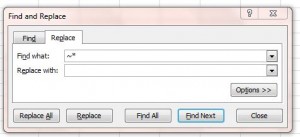
It’s a straightforward tool – there are a few options you can change when searching which I’ll save for a future blog post – but the post reminded me of my time in an office when we once needed to remove asterisks that had appeared in a set of data. My colleague’s first thought was to go straight to CTRL + H, activating the replace box and put * in the first box, leaving the second box blank, thus replacing it with nothing and in effect removing the pesky asterisks
But wait, what do you think happened? As * is used as a wildcard character to indicate any number of characters Excel assumed that they were looking for any characters and then removed them all, leaving a blank spreadsheet and a howling colleague. Quick use of CTRL + Z (undo) and the spreadsheet was returned to before.

The solution: before the asterisk in the “find what” box use a tilde sign ~ before the asterisk: ~* This tells Excel that it’s an actual * that is being searched for and is not being used as a wildcard.
This should also be used if searching and / or replacing for a question mark ( ? is used as a wildcard indicating a single character) and if you’re actually looking for a tilde you’ll need to have ~~ in the find what box.
Hope that this is helpful, more information is in a microsoft knowledgebase here.
Microsoft Excel Shortcut Tweet Roundup w/c 3rd October
Oct 7th
So this week’s Excel shortcut tweets turned out to be a celebration of F11:
______________________________________________________________________________________________
Insert a new worksheet SHIFT + F11
Delete the current sheet ALT + E then L
Activate Chart tool / wizard F11
Open VBA Editor ALT + F11
_______________________________________________________________________________________________
You may wonder what CTRL + F11 does. This inserts a new macro worksheet which is a relic back of the Excel4 days. Yes almost 20 years since Excel 4, when macros were written in a particular worksheet rather than the VBA editor, this shortcut still exists. As far as I know the new worksheets (titled Macro1 etc) don’t have any real use apart from for compatibility with the older version, unless you know to the contrary? Leave me a comment below as I’m intrigued if they’ve other uses.

Removing all hyperlinks from a spreadsheet
Sep 30th
The other day I retweeted a handy tip from Tom Urtis:
It can be frustrating if you have a large number of hyperlinks in an Excel spreadsheet which you want to remove as usually you’d have to go through each one individually to delete them all. This solution is a simple piece of VBA to go do them in bulk and is a great example of a quick piece of code as well as giving a few examples of handy shortcuts.
Make sure that you’ve got the spreadsheet open, with the active sheet being the one with the links on, then follow the steps above in Tom’s tweet. Broken down the shortcuts do the following:
_____________________________________________________________________________________
ALT + F11 Opens the VBA (Visual Basic for Applications) Editor.
CTRL + G Displays the Immediate Window, a place used often for debugging macros, but in this case a handy way of executing a single code immediately.
Type: ActiveSheet.Hyperlinks.Delete Does exactly what it says – checks the active sheet for hyperlinks and then deletes them
Enter Executes the code
Alt+Q Closes the VBA editor
_____________________________________________________________________________________
You should be left with a sheet with no hyperlinks, just their values – be warned if you want to do this on more than one worksheet in the same Excel workbook you’ll need to repeat it and also that you can’t undo this using the standard CTRL + Z. Perhaps a good opportunity to use Save As?

An Excel problem – the case of the frozen worksheet
Jul 26th
I had a call last week from someone who was struggling with a slightly unusual problem with a spreadsheet and needed a bit of Excel Detective work.
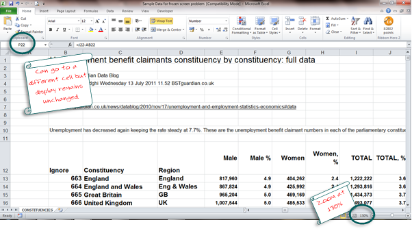
In this case the data wasn’t moving; nothing that he did would change the view he was seeing on the main worksheet. He had data in front of him when the file opened but as he moved the cursors around the screen the data remained still and didn’t scroll over to other rows or columns. He could use the cursors, or the go to command to move to different cells and could see data change in the name box and formula bar but on the main worksheet it was as if the screen was frozen.
Whilst on the call discussing possible causes he mentioned that the text seemed quite big and we worked out that the spreadsheet was displayed at zoomed up by 130%
From there it was quite straightforward to realise what had happened: the screen had been frozen so that the first few rows and first few columns remained visible. This is a simple, but very useful trick if you have large worksheets you wish to manoeuvre around. For example take a spreadsheet where the columns have heading labels in them, you may wish to freeze those so that as you scroll down the rows you can still which column contains what value.
In order to activate the freeze command then (using Excel 2010) click the View tab on the ribbon then click the freeze panes option:
You just then choose the one that you require – whether to freeze just the top row (you would likely use this if row 1 included your headers) or just the first column (or column A, for example if this was a list of names that you wanted to remain in view whilst you scrolled to the right)
If you choose the first option – freeze panes, this will freeze around whichever cell you have selected. For example if you’ve cell C3 selected it will keep frozen rows 1, 2 and 3 and columns A, B and C. All other cells you’ll be able to scroll through using your mouse, the cursor keys or whichever method you’d prefer.
If you’ve not used freeze panes it’s a really useful option, have a go on some of your own data.
Back to the ‘phone call. In this instance the freeze panes option had been used, afterwards someone had increased the scale of the zoom so rather than looking at the screen at 100% it was around 130% larger. I’m not sure if this was accidental or to make the text larger however the effect was that the frozen rows and columns were the only thing now visible on the screen, and the unfrozen rows and columns became hidden.
Excel was still working correctly – the problem was that there were no visible cells on the worksheet which weren’t frozen.
Excel Detective solution: return the zoom to 100% and / or unfreeze the panes,
A slightly unusual problem but a fun one to solve, have you come across anything similar? Use the comments below to let me know, I’d be interested to hear.


